How a Box Plot Example Reveals Hidden Data Patterns

The first time you encounter a box plot example in a dataset, it doesn’t just show numbers—it tells a story. Unlike bar charts that highlight averages or histograms that show frequency, a box plot compresses an entire distribution into a single frame, exposing skewness, spread, and anomalies in one glance. This is why financial analysts use box plot examples to detect market volatility, why quality control engineers rely on them to flag manufacturing defects, and why researchers prefer them over raw tables when presenting survey results. The power lies in its simplicity: five key components (median, quartiles, whiskers, and outliers) replace pages of statistical summaries.
Yet, many professionals overlook this tool because they assume it’s too abstract. In reality, a well-crafted box plot example can reveal patterns that even advanced statistical models might miss—particularly when comparing multiple groups or tracking changes over time. The secret isn’t memorizing formulas but understanding how the box’s length, the whiskers’ reach, and the dots beyond them interact. For instance, a symmetric box with equal whiskers suggests a normal distribution, while a lopsided box with a long upper whisker might indicate a ceiling effect in your data. These visual cues become intuitive once you’ve worked through practical box plot examples.
The versatility of box plots extends beyond academia. Sports analysts use them to compare player performance across seasons, healthcare professionals deploy them to assess treatment efficacy, and even urban planners rely on box plot examples to analyze income disparities by neighborhood. What makes them indispensable isn’t just their ability to summarize data but their capacity to spark questions—like why one quartile is unexpectedly wide or why outliers cluster in a specific range. The tool doesn’t just describe; it provokes deeper investigation.
The Complete Overview of Box Plot Examples
A box plot example is more than a graphical representation—it’s a statistical snapshot that distills complex datasets into actionable insights. At its core, it’s a five-number summary (minimum, first quartile, median, third quartile, and maximum) plotted against a numerical scale, with outliers marked separately. This design allows viewers to grasp distribution shape, central tendency, and variability in seconds. For example, in a box plot example comparing test scores across three schools, the median line’s position reveals which school performs best on average, while the box’s height shows consistency—narrow boxes indicate less variation, suggesting tighter grading curves.The real magic happens when you overlay multiple box plot examples side by side. Suddenly, you’re not just looking at numbers; you’re seeing relationships. Are the medians of two groups significantly different? Do the whiskers overlap, or is there a clear gap? These visual comparisons often uncover trends that numerical tables bury. For instance, a box plot example of customer satisfaction scores before and after a product redesign might show not just an improved median but also reduced spread, signaling both higher satisfaction and more consistent experiences. The tool’s strength lies in its balance: precise enough for technical analysis, intuitive enough for stakeholders without statistical backgrounds.
Historical Background and Evolution
The origins of the box plot trace back to 19th-century statistical pioneers, but its modern form was popularized by John Tukey in the 1960s as part of his work on exploratory data analysis (EDA). Tukey’s goal was to create a tool that could handle large datasets efficiently, and the box plot emerged as a solution to the limitations of histograms and stem-and-leaf plots. Early versions were crude—often hand-drawn on graph paper—but as computing power grew, software like R and Python’s `matplotlib` transformed them into dynamic, interactive box plot examples. Today, tools like Tableau and Excel’s built-in functions make it trivial to generate professional-grade visualizations with a few clicks.What makes the box plot’s evolution fascinating is its adaptability. Initially designed for univariate analysis, it was later extended to compare distributions across categories (notched box plots), handle time-series data (box plots with trend lines), and even incorporate probabilistic bounds (violins plots). The rise of big data hasn’t diminished its relevance; instead, it’s become a standard in dashboards where space is limited, and clarity is paramount. A box plot example in a 2023 data science report might include interactive tooltips, animations showing changes over time, or color-coding for multiple variables—yet the fundamental principles remain rooted in Tukey’s original design.
Core Mechanisms: How It Works
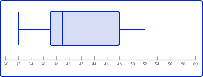
Understanding a box plot example requires dissecting its anatomy. The box itself represents the interquartile range (IQR), spanning from the first quartile (Q1, 25th percentile) to the third quartile (Q3, 75th percentile). The line inside the box marks the median (Q2, 50th percentile), revealing whether the distribution is skewed. Whiskers extend to 1.5 times the IQR beyond Q1 and Q3, capturing the bulk of the data; any points beyond these whiskers are flagged as outliers. This structure ensures that 50% of the data is always visible within the box, while the whiskers and outliers provide context for the tails.Table of Contents
- The Complete Overview of Box Plot Examples
- Historical Background and Evolution
- Core Mechanisms: How It Works
- Key Benefits and Crucial Impact
- Major Advantages
- Comparative Analysis
- Future Trends and Innovations
- Conclusion
- Comprehensive FAQs
- Q: What’s the difference between a box plot and a box-and-whisker plot?
- Q: How do I create a box plot example in Python?
- Q: Can box plots show negative values?
- Q: Why are outliers sometimes excluded from box plots?
- Q: How do I interpret a notched box plot?
- Q: Are box plots useful for time-series data?
- Q: What’s the best software for creating box plot examples?
- Q: How do box plots handle missing data?
- Q: Can box plots be used for categorical data?
- Q: What’s the most common mistake when creating box plot examples?
The genius of the box plot lies in its ability to standardize comparisons. For example, if you’re analyzing a box plot example of home prices in three cities, the width of each box tells you about price variability—narrow boxes suggest uniform pricing, while wide boxes indicate diverse markets. The position of the median relative to the box’s edges shows skewness: if the median is closer to Q1, the data is left-skewed (longer right whisker). Outliers, often plotted as individual dots, can be critical; in manufacturing, they might signal defective products, while in finance, they could indicate fraudulent transactions. The key is to interpret these elements holistically, not in isolation.
Key Benefits and Crucial Impact
Few visualization tools offer as much analytical depth in such a compact format as a box plot example. While scatter plots excel at showing correlations and line charts track trends, box plots specialize in revealing the underlying structure of distributions. This makes them indispensable in fields where understanding variability is critical—from clinical trials (assessing drug efficacy across patient groups) to supply chain management (monitoring delivery times). The ability to compare multiple distributions side by side with minimal cognitive load is unmatched. A single glance at a box plot example can reveal whether two datasets are statistically similar, identify which group has the most consistent performance, or pinpoint where outliers might warrant further investigation.The impact of box plots extends beyond efficiency; they democratize data interpretation. A well-designed box plot example can bridge the gap between technical analysts and non-technical stakeholders. For instance, a marketing team might use box plots to show how customer engagement varies by demographic without needing to explain standard deviations. Similarly, a box plot example of employee productivity scores across departments can highlight disparities that might prompt HR interventions. The tool’s clarity ensures that decisions aren’t delayed by statistical jargon, making it a cornerstone of data-driven cultures.
"A box plot is like a fingerprint for your data—it doesn’t just show you the numbers; it tells you the story behind them." — John Tukey, Statistician and EDA Pioneer
Major Advantages
- Compact yet informative: Condenses an entire dataset’s distribution into five key metrics, making it ideal for presentations and reports where space is limited.
- Outlier detection: Clearly marks data points that deviate significantly from the rest, helping identify anomalies that might require investigation.
- Comparative insights: Enables direct comparison of multiple groups or time periods, revealing patterns that raw numbers or histograms might obscure.
- Robustness to sample size: Works effectively with small datasets (e.g., survey responses) and large ones (e.g., sensor data), unlike tools sensitive to sample size.
- Non-parametric approach: Doesn’t assume a specific distribution (e.g., normality), making it reliable for real-world data that often violates statistical assumptions.

Comparative Analysis
| Box Plot | Alternative Visualizations |
|---|---|
|
|
Future Trends and Innovations
As data volumes grow and interactive tools become standard, box plot examples are evolving beyond static images. Modern implementations now incorporate dynamic filtering—allowing users to drill down into specific quartiles or outliers with a click. Machine learning is also enhancing box plots by automatically flagging "interesting" outliers (e.g., fraudulent transactions) or suggesting optimal bin sizes for better visualization. In the near future, we might see box plots integrated with predictive models, where the visualization not only describes past data but also forecasts future distributions based on trends.Another frontier is the fusion of box plots with other visualization types. For example, a "box-and-whisker" plot combined with a heatmap could show both distribution and correlation strength across variables. As augmented reality (AR) gains traction, imagine overlaying a box plot example in real-world contexts—like a construction site where workers see material defect rates visualized in AR glasses. The tool’s adaptability ensures it won’t become obsolete; instead, it will continue to redefine how we explore and interpret data.
Conclusion
The box plot’s enduring relevance stems from its ability to balance precision with simplicity. Whether you’re analyzing a box plot example of stock market returns, patient recovery times, or social media engagement metrics, the tool delivers insights that other visualizations can’t match. Its strength lies in exposing what matters most: not just the average but the spread, the skewness, and the outliers that often hold the most critical stories. As data literacy becomes a global priority, mastering the box plot isn’t just a technical skill—it’s a way to see the world more clearly.For professionals, the takeaway is clear: don’t treat box plot examples as static charts. Use them as a starting point for deeper questions. Why is this quartile wider than expected? What do these outliers represent? The best analysts don’t stop at the visualization—they let it guide their next steps. In an era drowning in data, the box plot remains one of the most powerful tools to cut through the noise and find meaning.
Comprehensive FAQs
Q: What’s the difference between a box plot and a box-and-whisker plot?
A box-and-whisker plot is essentially another name for a box plot. Both terms refer to the same visualization, which includes the box (IQR), median line, whiskers, and outliers. The distinction is purely semantic—some fields (like education) use "box-and-whisker," while others (like data science) prefer "box plot."
Q: How do I create a box plot example in Python?
Use the `seaborn` or `matplotlib` libraries. For a basic example:
import seaborn as sns
For customization (e.g., notched plots), add parameters like `notch=True` or `whis=1.0` to adjust whisker length.
sns.boxplot(data=df, x='category', y='values')
Q: Can box plots show negative values?
Yes. Box plots handle negative values naturally—they simply extend the whiskers and box below zero if the data includes them. For example, a box plot example of temperature data might show negative values for winter months.
Q: Why are outliers sometimes excluded from box plots?
Outliers are often plotted separately (as dots) rather than included in the whiskers to avoid skewing the perception of the dataset’s central tendency. The whiskers typically extend to 1.5×IQR, so points beyond that are considered outliers. Excluding them helps focus on the "typical" range of the data.
Q: How do I interpret a notched box plot?
A notched box plot adds a "notch" around the median to provide a rough confidence interval for the median. If notches of two boxes don’t overlap, it suggests the medians are significantly different (typically at the 5% level). This is useful for comparing groups, like testing scores across schools.
Q: Are box plots useful for time-series data?
Standard box plots aren’t ideal for time-series because they don’t show trends over time. However, you can create a "box plot over time" by generating separate box plots for each time period (e.g., monthly sales) and arranging them sequentially. Tools like `plotly` support interactive versions where you can hover over boxes to see exact values.
Q: What’s the best software for creating box plot examples?
For professionals, Python (`matplotlib`, `seaborn`), R (`ggplot2`), and Excel (via the "Insert Chart" tool) are top choices. For non-technical users, Tableau or Google Sheets offer drag-and-drop box plot creation. Advanced users might prefer specialized tools like Plotly for interactive visualizations.
Q: How do box plots handle missing data?
Box plots ignore missing values by default—they only plot the available data points. If missingness is systematic (e.g., certain groups have more missing data), it can bias the visualization. Always check for missing data patterns before interpreting a box plot example. Libraries like `pandas` in Python can help handle missing values before plotting.
Q: Can box plots be used for categorical data?
Indirectly, yes. Box plots are typically used for numerical data, but you can compare distributions across categories (e.g., "male vs. female income") by creating separate box plots for each category. The categories become the x-axis labels, while the y-axis shows the numerical variable.
Q: What’s the most common mistake when creating box plot examples?
The most frequent error is misinterpreting whiskers as representing the full range of data. Whiskers only extend to 1.5×IQR, so data beyond that (outliers) is excluded. Another mistake is ignoring the scale—box plots should always use a linear y-axis to avoid distorting perceptions of spread.
Leave a Comment
Comments are moderated before appearing. The data you submit is processed according to the Privacy Policy of Sac.