The Definitive Guide to How to Graph an Exponential Function
Exponential functions are the silent architects of growth and decay in nature, finance, and technology. Whether modeling population explosions, radioactive decay, or compound interest, their graphs reveal patterns invisible to linear or polynomial models. The ability to accurately plot these curves isn’t just academic—it’s a skill that bridges abstract theory with tangible outcomes. Yet, for many learners, the transition from algebraic manipulation to visual representation remains a stumbling block. The key lies in understanding the interplay between the function’s parameters and its graphical behavior, a nuance often overshadowed by rote memorization.
At its core, how to graph an exponential function hinges on three pillars: the base’s value, the horizontal shift, and the vertical scaling. A misstep in interpreting these elements can distort the entire curve, leading to misguided predictions in fields ranging from epidemiology to economics. The exponential function’s defining feature—its asymptotic behavior—demands a different approach than linear or quadratic graphs. Here, symmetry gives way to unbounded growth or decay, and the x-axis becomes an invisible barrier that the curve approaches but never crosses. Mastering this requires more than plotting points; it demands an intuitive grasp of limits and transformations.
The exponential function’s ubiquity isn’t accidental. From the spread of viruses to the depreciation of assets, its mathematical elegance mirrors the chaotic yet predictable rhythms of the natural world. Yet, despite its prevalence, confusion persists. Students often conflate exponential growth with linear trends, mistaking steady increments for multiplicative scaling. The result? Graphs that misrepresent reality. To avoid this pitfall, one must dissect the function’s components—base, exponent, and transformations—and observe how each alters the curve’s trajectory. This is where the art of graphing meets the rigor of mathematics.
The Complete Overview of How to Graph an Exponential Function
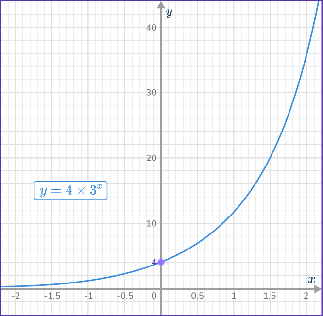
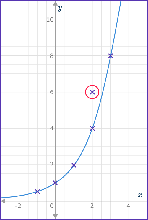
The exponential function, typically expressed as \( f(x) = a \cdot b^x \), where \( a \) and \( b \) are constants, serves as the foundation for modeling scenarios where quantities change by a consistent percentage over equal intervals. Unlike linear functions, which progress at a constant rate, exponential functions accelerate or decelerate dramatically, depending on whether \( b > 1 \) (growth) or \( 0 < b < 1 \) (decay). The graph of such a function is not a straight line but a curve that either ascends toward infinity or descends toward zero, asymptotically approaching the x-axis as \( x \) moves in the opposite direction. Understanding how to graph an exponential function thus begins with recognizing these fundamental behaviors: the horizontal asymptote, the y-intercept, and the rate of change dictated by the base \( b \).To plot an exponential function accurately, one must first identify its key features: the y-intercept (where \( x = 0 \)), the horizontal asymptote (the value \( f(x) \) approaches as \( x \) tends to negative infinity), and the end behavior (whether the function grows without bound or decays toward zero). The y-intercept is straightforward: when \( x = 0 \), \( f(0) = a \), meaning the graph crosses the y-axis at \( (0, a) \). The horizontal asymptote, however, is \( y = 0 \) for standard exponential functions, though transformations can shift this. The base \( b \) dictates the steepness of the curve—larger values of \( b \) produce steeper growth, while fractional bases (e.g., \( b = \frac{1}{2} \)) result in rapid decay. These elements collectively define the function’s shape, making how to graph an exponential function a process of translating algebraic properties into visual form.
Historical Background and Evolution
The exponential function’s origins trace back to the 17th century, when mathematicians like John Napier and Leonhard Euler sought to formalize the concept of continuous growth. Napier’s work on logarithms in 1614 laid the groundwork, revealing the inverse relationship between exponential and logarithmic functions—a discovery that would later simplify complex calculations in astronomy and navigation. By the 18th century, Euler’s introduction of the natural exponential function \( e^x \) (where \( e \approx 2.71828 \)) provided a universal tool for modeling natural phenomena, from cooling objects to bacterial growth. The graphing of these functions evolved alongside advancements in calculus, as mathematicians like Isaac Newton and Gottfried Wilhelm Leibniz recognized their utility in solving differential equations.The exponential function’s graphical representation became particularly significant in the 19th and 20th centuries, as scientists and engineers applied it to fields like physics, biology, and economics. The advent of computers in the mid-20th century further democratized access to exponential graphs, allowing for real-time modeling of everything from stock markets to pandemic spread. Today, how to graph an exponential function is not just a mathematical exercise but a critical skill in data-driven decision-making. The ability to visualize exponential trends—whether in climate science or financial forecasting—has become indispensable, reflecting the function’s enduring relevance across disciplines.
Core Mechanisms: How It Works
The exponential function’s graph is governed by its algebraic structure, where the variable \( x \) appears in the exponent. This distinction from polynomial functions, where \( x \) is the base, fundamentally alters the graph’s behavior. For \( f(x) = b^x \), the function’s value at any point \( x \) is determined by multiplying the base \( b \) by itself \( x \) times. When \( b > 1 \), each increment in \( x \) multiplies the output by \( b \), leading to exponential growth. Conversely, when \( 0 < b < 1 \), the output shrinks by a factor of \( b \) with each step, resulting in decay. The graph’s steepness is thus a direct consequence of the base’s magnitude, with larger \( b \) values producing more pronounced curvature.Table of Contents
- The Complete Overview of How to Graph an Exponential Function
- Historical Background and Evolution
- Core Mechanisms: How It Works
- Key Benefits and Crucial Impact
- Major Advantages
- Comparative Analysis
- Future Trends and Innovations
- Conclusion
- Comprehensive FAQs
- Q: What is the difference between exponential growth and exponential decay?
- Q: How do transformations affect the graph of an exponential function?
- Q: Why does an exponential function have a horizontal asymptote?
- Q: Can an exponential function ever be negative?
- Q: What real-world applications rely on graphing exponential functions?
- Q: How do I determine the base \( b \) of an exponential function from its graph?
- Q: What software tools can help graph exponential functions?
Transformations further refine the graph’s appearance. Vertical shifts (adding or subtracting a constant to the function) move the graph up or down, while horizontal shifts (replacing \( x \) with \( x - h \)) shift it left or right. Vertical stretches or compressions (multiplying the function by a constant) alter the amplitude, and reflections (negating the function) flip it over the x-axis. These transformations preserve the exponential function’s core properties—its horizontal asymptote and end behavior—while adjusting its position and scale. To graph an exponential function with transformations, one must systematically apply these changes, ensuring the curve retains its defining characteristics while adapting to new parameters.
Key Benefits and Crucial Impact
The exponential function’s graphical representation is more than a theoretical exercise; it is a practical tool for interpreting real-world data. In finance, for instance, compound interest follows an exponential pattern, where investments grow at a rate proportional to their current value. Graphing such functions allows investors to visualize long-term projections, identifying optimal growth strategies. Similarly, in epidemiology, exponential models describe the early stages of an outbreak, where the number of cases multiplies rapidly. Public health officials rely on these graphs to anticipate resource needs and implement containment measures before the curve becomes unmanageable. The ability to graph an exponential function thus translates mathematical abstraction into actionable insights.Beyond its applied uses, the exponential graph serves as a pedagogical cornerstone, illustrating concepts like limits, asymptotes, and nonlinear growth. Students who master these visualizations develop a deeper understanding of calculus and differential equations, fields where exponential functions frequently appear. Moreover, the graph’s intuitive representation of unbounded behavior fosters critical thinking about infinity and convergence—abstract ideas that become tangible through visual analysis. In an era where data literacy is paramount, the skills acquired through how to graph an exponential function extend far beyond the classroom, equipping individuals to navigate complex systems with confidence.
"The exponential function is the only one which takes small causes and gives large effects." — Pierre-Simon Laplace
Major Advantages
- Precision in Modeling: Exponential graphs accurately represent scenarios where growth or decay accelerates over time, such as bacterial cultures or radioactive decay. Their curvature reflects the multiplicative nature of these processes, unlike linear models that assume constant rates.
- Predictive Power: By plotting exponential functions, analysts can forecast future trends with greater accuracy. For example, in technology adoption, exponential curves often describe the diffusion of innovations, helping businesses anticipate market saturation.
- Visual Clarity: The graph’s distinct shape—either soaring upward or plunging toward zero—makes exponential trends immediately recognizable. This clarity aids in communicating complex data to non-experts, from policymakers to investors.
- Versatility: Exponential functions can be transformed to fit a wide range of datasets, from logarithmic scales in seismology to sigmoid curves in machine learning. Their adaptability makes them indispensable in interdisciplinary research.
- Foundation for Advanced Math: Mastery of exponential graphs is essential for studying calculus, differential equations, and probability theory. These fields rely on exponential functions to model rates of change and solve dynamic systems.
Comparative Analysis
| Exponential Function (\( f(x) = a \cdot b^x \)) | Linear Function (\( f(x) = mx + c \)) |
|---|---|
| Growth/decay accelerates multiplicatively (e.g., 2%, 4%, 8% per period). | Growth/decay is constant (e.g., +2 units per period). |
| Horizontal asymptote at \( y = 0 \) (unless transformed). | No asymptotes; extends infinitely in both directions. |
| Used for modeling population growth, compound interest, and decay processes. | Used for modeling steady trends, such as linear depreciation or uniform motion. |
| Graph is a curve with increasing/decreasing steepness. | Graph is a straight line with constant slope. |
Future Trends and Innovations
As data science and artificial intelligence continue to evolve, the role of exponential functions in modeling complex systems will expand. Machine learning algorithms, for instance, increasingly rely on exponential transformations to optimize loss functions and accelerate convergence in neural networks. The ability to graph an exponential function within these frameworks will become even more critical, as researchers seek to visualize the training dynamics of deep learning models. Similarly, in climate science, exponential decay models are being refined to predict the half-life of greenhouse gases, informing policy decisions with greater precision.Emerging fields like bioinformatics and quantum computing also leverage exponential functions to model probabilistic processes and algorithmic efficiency. For example, Shor’s algorithm, which threatens classical encryption, exploits exponential speedups in factoring large numbers. As these technologies mature, the graphical representation of exponential behavior will serve as a bridge between abstract theory and practical implementation. Educators and practitioners alike must therefore prioritize how to graph an exponential function not as an isolated skill, but as a gateway to understanding the exponential trends shaping the future.

Conclusion
The exponential function’s graph is a testament to mathematics’ power to capture the essence of dynamic systems. From the microscopic scale of chemical reactions to the macroscopic trends of global economies, its curves tell stories of growth, decay, and transformation. Learning how to graph an exponential function is more than a technical exercise; it is an invitation to see the world through a mathematical lens, where patterns emerge from chaos and predictions become possible. As technology advances, the demand for professionals who can interpret and manipulate these graphs will only grow, underscoring their relevance in an increasingly data-driven society.For students and practitioners alike, the journey to mastery begins with a single curve—a function that starts at a point, bends toward infinity, and leaves an indelible mark on the landscape of mathematics. By embracing the nuances of exponential graphs, one gains not just a tool, but a perspective: one that reveals the hidden order beneath the surface of exponential change.
Comprehensive FAQs
Q: What is the difference between exponential growth and exponential decay?
A: Exponential growth occurs when the base \( b \) of the function \( f(x) = b^x \) is greater than 1 (e.g., \( b = 2 \)), causing the output to increase rapidly as \( x \) rises. Exponential decay happens when \( 0 < b < 1 \) (e.g., \( b = 0.5 \)), leading the output to shrink toward zero. The graph of growth ascends steeply, while decay descends asymptotically toward the x-axis.
Q: How do transformations affect the graph of an exponential function?
A: Transformations shift, stretch, or reflect the graph while preserving its exponential nature. Vertical shifts (e.g., \( f(x) + k \)) move the graph up or down, while horizontal shifts (e.g., \( f(x - h) \)) shift it left or right. Vertical stretches/compressions (e.g., \( a \cdot f(x) \)) adjust the amplitude, and reflections (e.g., \( -f(x) \)) flip the graph over the x-axis. Each transformation alters specific features (e.g., asymptotes, intercepts) without changing the core exponential behavior.
Q: Why does an exponential function have a horizontal asymptote?
A: The horizontal asymptote of \( f(x) = b^x \) is \( y = 0 \) because as \( x \) approaches negative infinity, \( b^x \) (where \( b > 0 \)) approaches zero. This occurs because dividing a number by itself repeatedly (for negative \( x \)) yields values that shrink toward zero. Transformations (e.g., vertical shifts) can move this asymptote but never eliminate it.
Q: Can an exponential function ever be negative?
A: No, the standard exponential function \( f(x) = b^x \) (with \( b > 0 \)) always yields positive outputs. However, transformations like reflections (e.g., \( f(x) = -b^x \)) can produce negative values, flipping the graph over the x-axis. In such cases, the horizontal asymptote remains at \( y = 0 \), but the curve lies entirely below it.
Q: What real-world applications rely on graphing exponential functions?
A: Graphing exponential functions is critical in fields like finance (compound interest), biology (population growth), physics (radioactive decay), and epidemiology (disease spread). For example, in finance, exponential graphs help visualize how investments grow over time, while in medicine, they model the early stages of an epidemic before interventions alter the trend.
Q: How do I determine the base \( b \) of an exponential function from its graph?
A: To find \( b \), identify two points on the graph and solve for \( b \) using the equation \( f(x) = a \cdot b^x \). For instance, if the graph passes through (0, 2) and (1, 6), set \( 2 = a \cdot b^0 \) (so \( a = 2 \)) and \( 6 = 2 \cdot b^1 \), yielding \( b = 3 \). Alternatively, use the slope of the tangent line at \( x = 0 \), which equals \( a \cdot \ln(b) \).
Q: What software tools can help graph exponential functions?
A: Tools like Desmos, GeoGebra, and Python’s Matplotlib allow users to input exponential functions and visualize their graphs instantly. These platforms also support transformations and parameter adjustments, making it easier to explore how changes in \( a \) or \( b \) affect the curve. For advanced analysis, calculus software like Mathematica or Wolfram Alpha can compute limits and asymptotes dynamically.
Leave a Comment
Comments are moderated before appearing. The data you submit is processed according to the Privacy Policy of Sac.