How Simulated Annealing Solves Optimization Problems Like a Master Strategist
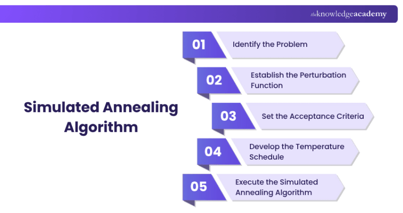
Every engineer, physicist, or data scientist who has grappled with optimization problems knows the frustration of being trapped by local optima—solutions that seem good enough but are far from the best possible outcome. Traditional methods like gradient descent can stumble here, unable to escape the gravitational pull of suboptimal peaks. That’s where simulated annealing steps in, borrowing a counterintuitive principle from metallurgy: controlled chaos. By simulating the slow cooling of molten metal—where atoms rearrange to form a stable crystal lattice—this probabilistic technique allows systems to "jump" out of poor solutions, even if they temporarily worsen the objective function. The result? A method that doesn’t just find solutions, but better ones, with applications spanning circuit design, logistics, and even protein folding.
The beauty of simulated annealing lies in its simplicity disguised as sophistication. Unlike brute-force searches that exhaustively test every possibility, it intelligently balances exploration and exploitation. At high "temperatures," the algorithm explores widely, accepting worse solutions to avoid premature convergence. As it cools, it refines its search, narrowing in on the global optimum with a precision that deterministic methods envy. This duality—between randomness and structure—makes it a cornerstone of metaheuristic optimization, a field where creativity meets computational rigor.
Yet for all its elegance, simulated annealing remains misunderstood. Many associate it with niche academic exercises, unaware of its real-world dominance in solving NP-hard problems—from routing delivery trucks to tuning neural networks. The technique’s adaptability extends beyond pure optimization; it’s a philosophy of problem-solving that prioritizes resilience over rigidity. In an era where data complexity is exploding, understanding how to harness this method isn’t just useful—it’s essential.
The Complete Overview of Simulated Annealing
Simulated annealing is a probabilistic optimization algorithm designed to approximate global solutions to complex problems by mimicking the physical process of annealing in metallurgy. In materials science, annealing involves heating a material to a high temperature and then slowly cooling it to reduce defects and improve its properties. Similarly, the algorithm begins with a high "temperature" parameter that allows it to explore a wide range of potential solutions, including those that are worse than the current best. As the temperature decreases, the algorithm becomes more selective, favoring better solutions while still permitting occasional escapes from local optima. This gradual cooling process ensures convergence toward a globally optimal—or near-optimal—solution.
The algorithm’s core innovation lies in its ability to escape local minima, a limitation plaguing many optimization techniques. By incorporating a probabilistic acceptance criterion—where worse solutions are accepted with a probability that diminishes as the temperature drops—simulated annealing effectively balances exploration and exploitation. This duality is what sets it apart from deterministic methods, which risk getting stuck in suboptimal regions of the solution space. Developed in the early 1980s by Kirkpatrick, Gelatt, and Vecchi, the method was initially applied to circuit design but quickly gained traction across disciplines, from operations research to bioinformatics.
Historical Background and Evolution
The origins of simulated annealing trace back to the 1950s, when physicists like Metropolis and colleagues introduced the Metropolis-Hastings algorithm to study statistical mechanics. This algorithm, which simulates the behavior of particles in a thermal system, laid the groundwork for probabilistic optimization. However, it wasn’t until 1983 that simulated annealing was formally adapted for combinatorial optimization by Saul Kirkpatrick, Carlo Gelatt, and Mario Vecchi. Their paper, "Optimization by Simulated Annealing," demonstrated how the annealing process could be repurposed to solve the traveling salesman problem—a classic NP-hard challenge—by treating the problem’s energy landscape analogously to the physical system’s free energy.
Table of Contents
- The Complete Overview of Simulated Annealing
- Historical Background and Evolution
- Core Mechanisms: How It Works
- Key Benefits and Crucial Impact
- Major Advantages
- Comparative Analysis
- Future Trends and Innovations
- Conclusion
- Comprehensive FAQs
- Q: How does simulated annealing differ from genetic algorithms?
- Q: What is the role of the cooling schedule in simulated annealing?
- Q: Can simulated annealing be applied to continuous optimization problems?
- Q: Why is simulated annealing called "simulated" annealing?
- Q: What are the main challenges in implementing simulated annealing?
- Q: How is simulated annealing used in machine learning?
- Q: Are there any real-world industries where simulated annealing is widely used?
Since its inception, the technique has evolved through refinements in cooling schedules, neighborhood structures, and adaptive parameters. Early implementations used fixed cooling rates, but modern variants incorporate dynamic adjustments, such as adaptive temperature scaling or restart mechanisms, to improve efficiency. Today, simulated annealing is not just a standalone algorithm but a foundational concept in metaheuristic optimization, influencing derivatives like genetic algorithms and particle swarm optimization. Its adaptability has also led to hybrid approaches, where it’s combined with gradient-based methods or machine learning to tackle problems where no single technique suffices.
Core Mechanisms: How It Works
At its heart, simulated annealing operates on three key components: an initial solution, a neighborhood function, and a cooling schedule. The algorithm starts with a randomly generated or heuristically chosen solution, which is then iteratively perturbed by a neighborhood function—typically a small, random change to the current solution (e.g., swapping two cities in a route). The critical step is evaluating whether to accept this new solution. If it’s better than the current one, it’s always accepted. If it’s worse, it’s accepted with a probability that depends on the current "temperature" and the difference in objective values, governed by the Boltzmann distribution: \( P(\Delta E) = e^{-\Delta E / T} \), where \( \Delta E \) is the change in the objective function and \( T \) is the temperature.
The temperature parameter is the algorithm’s thermostat, controlling the trade-off between exploration and exploitation. Initially set high, it allows the algorithm to explore broadly, accepting poor solutions to avoid premature convergence. As the temperature decreases according to a predefined schedule (e.g., exponential or logarithmic cooling), the probability of accepting worse solutions diminishes, and the algorithm focuses on refining the best-known solution. The cooling schedule is crucial: too fast, and the algorithm may converge to a local optimum; too slow, and it risks wasting computational resources. The choice of schedule often depends on the problem’s complexity and the desired balance between speed and solution quality.
Key Benefits and Crucial Impact
Simulated annealing revolutionized optimization by addressing a fundamental limitation of deterministic methods: their inability to escape local optima. Traditional approaches like hill climbing or gradient descent are prone to getting trapped in suboptimal regions of the solution space, especially in problems with many variables or constraints. By introducing controlled randomness, simulated annealing transforms optimization into a dynamic process where the algorithm can "climb out" of poor solutions, even if it means temporarily moving backward. This flexibility makes it particularly effective for NP-hard problems, where exhaustive searches are computationally infeasible.
The algorithm’s impact extends beyond theoretical advantages. In practice, simulated annealing has been deployed in industries where precision and adaptability are critical. For instance, in VLSI (very-large-scale integration) circuit design, it optimizes chip layouts to minimize wire length and power consumption. In logistics, it streamlines delivery routes, reducing costs and fuel consumption. Even in bioinformatics, it aids in protein folding simulations, where the energy landscape is notoriously rugged. Its versatility stems from its problem-agnostic nature: as long as an objective function and neighborhood structure can be defined, simulated annealing can be applied.
"Simulated annealing is not just an algorithm; it’s a metaphor for intelligent problem-solving—a reminder that sometimes, the path to the best solution requires embracing temporary setbacks."
—Saul Kirkpatrick, Co-developer of Simulated Annealing
Major Advantages
- Global Optimization Capability: Unlike local search methods, simulated annealing is designed to escape local minima, increasing the likelihood of finding a globally optimal or near-optimal solution.
- Adaptability: The algorithm can be applied to a wide range of problems, from continuous to discrete, as long as a neighborhood structure and objective function are defined.
- Flexibility in Cooling Schedules: The choice of cooling rate allows users to balance exploration and exploitation, tailoring the algorithm to specific problem requirements.
- Robustness to Noise: The probabilistic nature of the algorithm makes it resilient to minor fluctuations in the objective function, which is beneficial in real-world scenarios with uncertain data.
- Theoretical Guarantees: Under certain conditions, simulated annealing can converge to the global optimum with probability 1, provided the cooling schedule is sufficiently slow.

Comparative Analysis
While simulated annealing excels in many scenarios, it’s not universally superior. Understanding its strengths and weaknesses relative to other optimization techniques is essential for selecting the right tool. Below is a comparative overview of simulated annealing against three other prominent methods:
| Criteria | Simulated Annealing | Genetic Algorithms | Gradient Descent |
|---|---|---|---|
| Optimization Type | Global (probabilistic) | Global (population-based) | Local (deterministic) |
| Escape from Local Minima | High (via temperature control) | Moderate (via crossover/mutation) | Low (prone to trapping) |
| Computational Complexity | High (depends on cooling schedule) | High (population size and generations) | Low (but limited to smooth functions) |
| Best Use Case | NP-hard problems, combinatorial optimization | Multi-modal, discrete problems | Differentiable, convex problems |
Simulated annealing’s probabilistic approach makes it a strong candidate for problems where the solution space is vast and discontinuous, such as scheduling or network design. However, for problems with smooth, differentiable objective functions, gradient descent remains the faster choice. Genetic algorithms, which operate on populations of solutions, can outperform simulated annealing in problems with multiple optima but require careful tuning of parameters like mutation rates and crossover strategies.
Future Trends and Innovations
The future of simulated annealing lies in its integration with emerging technologies and adaptive enhancements. One promising direction is the development of adaptive simulated annealing, where the cooling schedule and acceptance criteria are dynamically adjusted based on real-time performance metrics. Machine learning is also playing a role, with researchers exploring how neural networks can optimize annealing parameters or even replace traditional neighborhood functions with learned perturbations. These hybrid approaches aim to reduce the algorithm’s sensitivity to initial conditions and improve convergence rates.
Another frontier is the application of simulated annealing in quantum computing. Quantum annealing, a variant of the algorithm, leverages quantum mechanics to explore solution spaces exponentially faster than classical methods. Companies like D-Wave are already deploying quantum annealers for optimization problems in finance, chemistry, and AI. As quantum hardware matures, classical simulated annealing may evolve into a bridge between today’s computational limitations and tomorrow’s quantum advantages. Additionally, the rise of edge computing could democratize simulated annealing, enabling real-time optimization in IoT devices and autonomous systems where latency is critical.

Conclusion
Simulated annealing stands as a testament to the power of borrowing principles from nature to solve human-made problems. Its ability to transform a seemingly chaotic process—controlled randomness—into a structured optimization framework has made it indispensable in fields where precision and adaptability are paramount. While it may not be the fastest or most straightforward method for every problem, its robustness in escaping local optima and its broad applicability ensure its relevance in an era of increasing data complexity.
As optimization problems grow more intricate—driven by advancements in AI, big data, and quantum computing—the principles of simulated annealing will continue to inspire innovation. Whether through adaptive variants, hybrid algorithms, or quantum implementations, the core idea remains unchanged: sometimes, the best way forward is to embrace a little disorder. For practitioners and researchers alike, understanding and leveraging simulated annealing is not just about solving problems—it’s about rethinking how problems are approached.
Comprehensive FAQs
Q: How does simulated annealing differ from genetic algorithms?
A: While both are metaheuristic optimization techniques, simulated annealing operates on a single solution at a time, using temperature-controlled randomness to escape local optima. Genetic algorithms, on the other hand, maintain a population of solutions that evolve through selection, crossover, and mutation. Simulated annealing is often more efficient for fine-tuning a single solution, whereas genetic algorithms excel in exploring diverse regions of the solution space.
Q: What is the role of the cooling schedule in simulated annealing?
A: The cooling schedule determines how the temperature parameter decreases over time, directly influencing the algorithm’s balance between exploration and exploitation. A schedule that cools too quickly may lead to premature convergence, trapping the algorithm in a local optimum. Conversely, a schedule that cools too slowly can result in excessive computational time without significant improvement. Common schedules include exponential, logarithmic, and adaptive cooling, each suited to different problem characteristics.
Q: Can simulated annealing be applied to continuous optimization problems?
A: Yes, simulated annealing is not limited to discrete or combinatorial problems. For continuous optimization, the neighborhood function can be defined using small, random perturbations to the current solution (e.g., adding Gaussian noise to variables). However, the effectiveness depends on the problem’s landscape; highly non-convex or noisy functions may require careful tuning of the temperature and step size parameters.
Q: Why is simulated annealing called "simulated" annealing?
A: The term "simulated" refers to the algorithm’s imitation of the physical annealing process in metallurgy, where a material is heated and then slowly cooled to reduce defects and achieve a stable, low-energy state. The "annealing" metaphor is used because the algorithm’s temperature parameter and acceptance criterion mimic the thermodynamic behavior of particles in a molten material, gradually settling into a more ordered (optimal) configuration.
Q: What are the main challenges in implementing simulated annealing?
A: The primary challenges include selecting an appropriate cooling schedule, defining an effective neighborhood structure, and choosing the initial temperature and step size. Poor choices can lead to slow convergence, local optima trapping, or excessive runtime. Additionally, tuning these parameters often requires domain knowledge or empirical testing, as there are no universal rules for all problem types. Hybrid approaches or automated tuning mechanisms can mitigate some of these challenges.
Q: How is simulated annealing used in machine learning?
A: In machine learning, simulated annealing is often employed for hyperparameter optimization, neural network training, and feature selection. For instance, it can optimize the weights of a neural network by treating the loss function as an energy landscape, allowing the algorithm to escape poor local minima during training. It’s also used in clustering algorithms, such as the annealing version of the k-means algorithm, to improve initialization and avoid suboptimal cluster assignments.
Q: Are there any real-world industries where simulated annealing is widely used?
A: Yes, simulated annealing has practical applications in several industries. In electronics, it optimizes VLSI circuit layouts and PCB design. In logistics and transportation, it solves vehicle routing and scheduling problems. The financial sector uses it for portfolio optimization and risk management. Even in biomedicine, it aids in drug design and protein folding simulations. Its versatility makes it a go-to tool for problems requiring global optimization in high-dimensional spaces.
Leave a Comment
Comments are moderated before appearing. The data you submit is processed according to the Privacy Policy of Sac.