Decoding the Inner Workings of Inner Join: SQL’s Hidden Powerhouse

Databases don’t just store data—they orchestrate relationships. At the heart of this orchestration lies the inner join, a foundational operation that filters results to only what matters: the intersection of two tables. Unlike its more permissive cousins (outer joins), it enforces precision, ensuring only matching records emerge. This selectivity is its superpower, but it also demands a nuanced understanding of how to wield it without unintended consequences.
The inner join isn’t just a syntax choice; it’s a design philosophy. It embodies the principle that data should be meaningful only when explicitly connected. Whether you’re stitching together customer orders with product inventories or merging user profiles with activity logs, the inner join acts as a gatekeeper, rejecting nulls and mismatches. Yet, its simplicity belies complexity: a poorly structured inner join can silently exclude critical data, turning a query into a black box of assumptions.
Behind every efficient database lies a series of inner join operations—some explicit, others hidden in views or stored procedures. Developers often treat it as a given, but its mechanics are worth dissecting. How does it traverse tables? What happens when join conditions are ambiguous? And why does it sometimes outperform alternatives like subqueries? These questions reveal the inner join as more than a tool: it’s a lens through which data relationships are clarified, optimized, and sometimes, unexpectedly, broken.
The Complete Overview of Inner Join
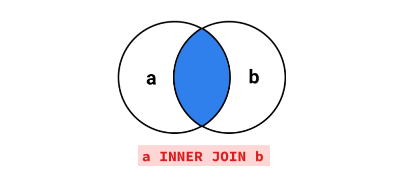
The inner join is the most fundamental relational operation in SQL, serving as the default when combining data from multiple tables. At its core, it performs a Cartesian product between two tables but then applies a join condition to filter results, retaining only rows where the condition evaluates to true. This process ensures that every returned row has a corresponding match in both tables—a strict requirement that distinguishes it from outer joins, which include unmatched rows with null placeholders.
Understanding the inner join requires grasping two key concepts: the join condition (often using the `ON` clause) and the result set’s composition. The condition defines how rows are matched—typically via shared keys like foreign references—but it can also involve arbitrary expressions. The result set, meanwhile, combines columns from both tables, with the join condition implicitly dictating which combinations are valid. This interplay between structure and logic is why the inner join is both versatile and precise.
Historical Background and Evolution
The concept of joining tables emerged alongside relational databases in the 1970s, when Edgar F. Codd formalized the relational model. Early implementations, like IBM’s System R, introduced the idea of combining tables via common attributes, but the syntax for inner joins evolved significantly. The original SQL standard (1986) used the comma-separated join syntax, where tables were listed and conditions specified in the `WHERE` clause. This approach was error-prone, as it conflated filtering logic with join semantics.
Table of Contents
- The Complete Overview of Inner Join
- Historical Background and Evolution
- Core Mechanisms: How It Works
- Key Benefits and Crucial Impact
- Major Advantages
- Comparative Analysis
- Future Trends and Innovations
- Conclusion
- Comprehensive FAQs
- Q: Can an inner join return duplicate rows?
- Q: How does indexing affect inner join performance?
- Q: What happens if I join two tables with no matching rows?
- Q: Is there a performance difference between `INNER JOIN` and comma-separated joins with `WHERE`?
- Q: Can I use an inner join with more than two tables?
The modern `INNER JOIN` syntax, introduced in later SQL standards (e.g., SQL-92), clarified intent by separating join conditions from filtering. This change reflected a broader trend toward explicit, readable query structures. Today, the inner join is a cornerstone of SQL, supported by all major database systems (PostgreSQL, MySQL, Oracle, SQL Server) with consistent behavior across vendors. Its ubiquity stems from its balance of simplicity and power: it solves a common problem without unnecessary complexity.
Core Mechanisms: How It Works
When executed, an inner join follows a three-step process: table scanning, condition evaluation, and result assembly. The database engine first scans both tables, building temporary data structures (like hash tables or nested loops) to compare rows. The join condition is then evaluated for each potential pair, and only matching rows proceed to the final stage, where columns are combined into the result set. This process is optimized via query planners, which choose algorithms (e.g., hash join, merge join) based on table sizes and indexes.
The mechanics of the inner join are deceptively simple, but nuances arise in practice. For example, non-equijoins (joins with conditions like `>`, `<`) can produce unexpected results if not carefully crafted. Similarly, joining more than two tables (nested joins) requires careful ordering to avoid performance pitfalls. The engine’s ability to push predicates (filters) into the join process also affects efficiency, making indexing and query structure critical. Mastery of these mechanics ensures that the inner join remains both performant and predictable.
Key Benefits and Crucial Impact
The inner join’s primary advantage is its clarity: it explicitly declares which data relationships are relevant, eliminating ambiguity. This precision is invaluable in applications where data integrity is paramount, such as financial systems or healthcare records. By excluding unmatched rows, it reduces noise in results, allowing analysts to focus on valid combinations. Additionally, its performance characteristics—when properly optimized—make it a workhorse for large-scale data processing.
Beyond technical efficiency, the inner join aligns with relational theory, where data is organized into normalized tables with explicit links. This design minimizes redundancy and simplifies updates. However, its rigid matching can also be a drawback: if a table lacks expected records, the join silently drops them, potentially masking data issues. Balancing this trade-off requires understanding when to use inner joins versus alternatives like left joins or subqueries.
— Donald D. Chamberlin (co-creator of SQL)
"Joins are the glue that holds relational databases together. The inner join, in particular, enforces the very principle that data should be connected only when it makes sense."
Major Advantages
- Data Integrity: Ensures only valid, matched rows are returned, reducing errors from orphaned or mismatched records.
- Performance: Optimized join algorithms (e.g., hash joins) often outperform outer joins or subqueries for large datasets.
- Readability: Explicit syntax (`INNER JOIN table ON condition`) clarifies intent compared to implicit `WHERE` clause joins.
- Normalization Support: Aligns with relational design by enforcing referential integrity through matching keys.
- Flexibility: Can join on non-key columns or use complex conditions (e.g., `JOIN orders ON orders.date BETWEEN '2023-01-01' AND '2023-12-31'`).
Comparative Analysis
| Inner Join | Left Outer Join |
|---|---|
| Returns only rows with matches in both tables. | Returns all rows from the left table, with nulls for unmatched right-table rows. |
| Syntax: `INNER JOIN table ON condition` | Syntax: `LEFT JOIN table ON condition` |
| Use case: When unmatched rows are irrelevant. | Use case: When preserving all left-table rows is critical (e.g., reporting). |
| Performance: Often faster for large datasets with matches. | Performance: Slower due to additional null padding. |
Future Trends and Innovations
The inner join remains central to SQL, but its implementation is evolving with advancements in distributed databases and query optimization. Modern engines now leverage parallel processing to execute joins across sharded data, reducing latency in cloud environments. Additionally, machine learning-driven query planners are beginning to dynamically select join strategies, further optimizing performance without manual intervention.
Looking ahead, the rise of graph databases and polyglot persistence may reduce reliance on traditional joins, but the inner join’s principles—explicit relationships and filtered results—will persist in hybrid architectures. Tools like window functions and CTEs (Common Table Expressions) are also redefining how joins are composed, enabling more modular and maintainable queries. As data grows in complexity, the inner join’s role as a foundational operation will only solidify.

Conclusion
The inner join is more than a syntax construct; it’s a reflection of relational databases’ core philosophy: data should be connected meaningfully. Its ability to filter and combine tables with precision makes it indispensable, but its power requires careful handling. Misuse can lead to silent data loss, while overuse may obscure the underlying schema. The key lies in aligning join logic with the problem domain—whether that means enforcing strict matches or recognizing when outer joins are more appropriate.
As databases grow in scale and complexity, the inner join will continue to adapt, but its fundamental role as the standard for relational integration remains unchanged. For developers and analysts, understanding its mechanics isn’t just about writing queries—it’s about designing systems where data relationships are explicit, efficient, and reliable.
Comprehensive FAQs
Q: Can an inner join return duplicate rows?
A: No. By definition, an inner join returns each matching row pair exactly once, even if multiple rows in one table satisfy the join condition. Duplicates would only appear if the underlying tables contain duplicate keys or if the join condition is non-deterministic (e.g., joining on a non-unique column without aggregation).
Q: How does indexing affect inner join performance?
A: Indexes dramatically improve join performance by allowing the database engine to locate matching rows faster. For example, an index on the join column of the smaller table can reduce the join from O(n²) to O(n log n) in many cases. However, over-indexing can slow down writes, so indexes should target columns frequently used in joins or filters.
Q: What happens if I join two tables with no matching rows?
A: The result set will be empty. Unlike outer joins, an inner join has no mechanism to return unmatched rows; it strictly adheres to the "only matching pairs" rule. This behavior is intentional and can be leveraged to test for data completeness (e.g., `SELECT COUNT(*) FROM inner_join_result` to check for missing connections).
Q: Is there a performance difference between `INNER JOIN` and comma-separated joins with `WHERE`?
A: Modern SQL engines treat these syntactically equivalent, but explicit `INNER JOIN` syntax is preferred for readability and maintainability. The comma-separated style (e.g., `FROM table1, table2 WHERE table1.id = table2.id`) is considered legacy and can lead to confusion, especially in complex queries. Always use the explicit syntax for clarity.
Q: Can I use an inner join with more than two tables?
A: Yes, but the order of joins matters. The database evaluates joins left-to-right unless parentheses specify otherwise. For example, `A INNER JOIN B ON A.id = B.a_id INNER JOIN C ON B.id = C.b_id` joins `A` and `B` first, then joins the result with `C`. Parentheses can override this: `(A INNER JOIN B ON A.id = B.a_id) INNER JOIN C ON A.id = C.a_id` changes the grouping. Always test join order with `EXPLAIN` to verify performance.
Leave a Comment
Comments are moderated before appearing. The data you submit is processed according to the Privacy Policy of Sac.