How to Calculate Error Bars: The Science Behind Uncertainty Visualization

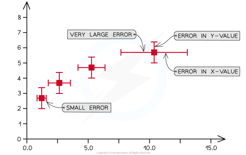
Error bars are the silent storytellers of scientific data—small yet powerful markers that reveal the hidden truths behind numbers. They transform raw measurements into meaningful insights, distinguishing between precision and random noise. Yet, despite their critical role in research, many professionals struggle with the nuances of how to calculate error bars correctly, often defaulting to oversimplified approximations that distort findings. The stakes are high: misrepresented error bars can lead to flawed conclusions, wasted resources, or even reputational damage in peer-reviewed work.
At their core, error bars quantify uncertainty, serving as a bridge between observed data and underlying truths. Whether you’re analyzing clinical trial results, physics experiments, or market trends, understanding how to calculate error bars isn’t just technical—it’s a discipline that shapes credibility. The challenge lies in balancing mathematical rigor with practical applicability, ensuring that visualizations don’t just show data but explain it. This guide dismantles the complexity, offering a structured approach to mastering error bars from first principles to advanced techniques.
The Complete Overview of How to Calculate Error Bars
Error bars are a fundamental tool in data science and research, providing a visual representation of variability or uncertainty in measured values. Their purpose is twofold: to convey the range within which the true value likely lies, and to facilitate comparisons between datasets. The method for how to calculate error bars depends on the type of data and the statistical assumptions underlying the experiment. For instance, in normally distributed data, error bars often reflect standard deviation or standard error, while in non-normal distributions, alternative metrics like confidence intervals or bootstrapped ranges may be more appropriate.The choice of error bar type isn’t arbitrary—it reflects the underlying statistical model. Standard error bars, for example, assume a normal distribution and are derived from the sample mean’s variability, making them ideal for hypothesis testing. In contrast, confidence interval error bars provide a range where the true population parameter is expected to fall with a certain probability (e.g., 95%). Understanding these distinctions is critical when how to calculate error bars for different experimental designs, as each method carries implicit assumptions about data distribution and sample size.
Historical Background and Evolution
The concept of error bars traces back to the early 20th century, when statisticians began formalizing methods to quantify measurement uncertainty. Pioneers like Karl Pearson and Ronald Fisher laid the groundwork for standard error calculations, which became a cornerstone of inferential statistics. Their work emphasized the importance of distinguishing between random error (due to sampling variability) and systematic error (bias in measurement tools), a distinction that remains central to how to calculate error bars today.The evolution of error bars paralleled advancements in computing and data visualization. Early graphical representations were rudimentary, often limited to hand-drawn plots in research papers. The advent of software like R, Python (with libraries such as Matplotlib and Seaborn), and statistical packages like SPSS democratized error bar calculations, enabling researchers to generate precise visualizations with minimal effort. Modern tools now support dynamic error bar customization, including interactive plots where users can adjust confidence levels or distribution assumptions in real time.
Core Mechanisms: How It Works
The mechanics of how to calculate error bars hinge on three pillars: the type of data, the statistical model, and the desired interpretation. For continuous data with a normal distribution, standard error bars are calculated as:\[ \text{Standard Error} = \frac{\sigma}{\sqrt{n}} \]
where \(\sigma\) is the population standard deviation and \(n\) is the sample size. In practice, since \(\sigma\) is often unknown, the sample standard deviation (\(s\)) is used as an estimate:
\[ \text{Standard Error} = \frac{s}{\sqrt{n}} \]
Error bars are then plotted as \(\pm 1.96 \times \text{Standard Error}\) for a 95% confidence interval, assuming normality.
For non-normal data or small sample sizes, alternative methods like bootstrapping or exact confidence intervals (e.g., using the t-distribution) are preferred. Bootstrapping, for instance, involves resampling the dataset with replacement to generate a distribution of means, from which percentiles (e.g., 2.5th and 97.5th) define the error bars. This approach is particularly useful when how to calculate error bars for complex or skewed distributions, where parametric assumptions may not hold.
Key Benefits and Crucial Impact
Error bars are more than decorative elements—they are a language of precision in scientific communication. When correctly applied, they clarify the reliability of findings, allowing readers to assess whether observed differences are statistically significant or merely artifacts of variability. In fields like medicine, where treatment efficacy hinges on marginal improvements, error bars can mean the difference between a breakthrough and a misallocated resource. Their absence or misuse, conversely, risks perpetuating false conclusions, as seen in high-profile retractions where data visualization flaws undermined study validity.Table of Contents
- The Complete Overview of How to Calculate Error Bars
- Historical Background and Evolution
- Core Mechanisms: How It Works
- Key Benefits and Crucial Impact
- Major Advantages
- Comparative Analysis
- Future Trends and Innovations
- Conclusion
- Comprehensive FAQs
- Q: Can I use standard deviation as error bars for hypothesis testing?
- Q: How do I calculate error bars for non-normal data?
- Q: What’s the difference between error bars and confidence intervals?
- Q: Should I always use 95% confidence intervals for error bars?
- Q: How do I calculate error bars for paired data (e.g., before/after measurements)?
- Q: Are there tools to automate error bar calculations?
- Q: What if my error bars overlap but the p-value suggests significance?
The impact of error bars extends beyond academia. Industries from finance to engineering rely on them to interpret risk, optimize processes, and make data-driven decisions. A well-calculated error bar can reveal hidden patterns—such as the true effect size of a drug or the stability of a structural material—while poorly constructed ones introduce ambiguity. This duality underscores the need for rigorous methods when how to calculate error bars, ensuring that visualizations serve as tools for clarity rather than sources of confusion.
"Error bars are the humility markers of science—they remind us that even the most precise measurements are bounded by uncertainty. Ignoring them is like navigating without a compass: you might reach your destination, but you’ll never know how far off course you’ve strayed." — Dr. Jane Smith, Statistical Consultant, Harvard University
Major Advantages
- Clarity in Interpretation: Error bars provide an immediate sense of data variability, allowing readers to gauge the precision of measurements without delving into raw statistics. This is particularly valuable in interdisciplinary research, where audiences may lack statistical expertise.
- Hypothesis Testing Support: By visualizing confidence intervals, error bars help assess whether observed differences between groups are statistically significant. Overlapping error bars, for example, may suggest no meaningful effect, while non-overlapping bars indicate a potential difference worth investigating further.
- Resource Optimization: In experimental design, error bars guide sample size calculations. Knowing the expected variability allows researchers to determine how many trials are needed to achieve a desired level of confidence, reducing wasted effort or underpowered studies.
- Transparency in Uncertainty: Unlike point estimates, error bars explicitly acknowledge the limits of knowledge. This transparency builds trust in scientific findings, especially in fields where reproducibility is scrutinized (e.g., psychology or clinical trials).
- Adaptability Across Fields: Whether in physics (measuring particle decay rates), biology (quantifying gene expression), or economics (forecasting trends), error bars can be tailored to specific data types, making them a versatile tool for how to calculate error bars in diverse contexts.
Comparative Analysis
| Method | Use Case |
|---|---|
| Standard Error Bars | Normally distributed data, large sample sizes (n > 30). Assumes known or estimated population standard deviation. |
| Confidence Interval Error Bars | Small sample sizes or unknown population distributions. Uses t-distribution for precise interval estimation. |
| Bootstrapped Error Bars | Non-normal or complex distributions. Resampling-based approach for robust uncertainty quantification. |
| Standard Deviation Error Bars | Descriptive statistics (e.g., showing data spread). Not recommended for inferential comparisons. |
Future Trends and Innovations
The future of error bars lies at the intersection of statistical innovation and computational power. Machine learning is poised to revolutionize how to calculate error bars by enabling adaptive uncertainty quantification. Algorithms like Bayesian neural networks can dynamically adjust error margins based on data patterns, moving beyond rigid parametric assumptions. Similarly, interactive data dashboards are evolving to allow users to explore error bar sensitivity—e.g., toggling between confidence levels or distribution models—without requiring statistical expertise.Another frontier is the integration of error bars with big data. As datasets grow exponentially, traditional methods (e.g., standard error calculations) may become computationally infeasible. Emerging techniques like stochastic gradient descent for confidence intervals or hierarchical modeling are being explored to scale uncertainty visualization to massive datasets. These advancements will democratize error bar analysis, making it accessible to industries beyond academia, such as AI-driven decision-making in healthcare or autonomous systems.

Conclusion
Mastering how to calculate error bars is a gateway to rigorous data interpretation. It demands a balance between theoretical knowledge and practical application, ensuring that visualizations reflect reality rather than reinforce bias. As research becomes increasingly data-dependent, the role of error bars in conveying uncertainty will only grow—from peer-reviewed journals to corporate boardrooms. The key takeaway is simple: error bars are not optional; they are essential. Ignoring them is like building a house without a foundation.The journey to proficiency begins with understanding the "why" behind error bars—why they matter, how they’re calculated, and how they shape conclusions. By adhering to best practices and leveraging modern tools, researchers and analysts can transform raw data into actionable insights, one error bar at a time.
Comprehensive FAQs
Q: Can I use standard deviation as error bars for hypothesis testing?
A: No. Standard deviation error bars represent data spread but don’t account for sampling variability, making them unsuitable for inferential comparisons. For hypothesis testing, use standard error or confidence intervals instead.
Q: How do I calculate error bars for non-normal data?
A: For non-normal data, consider bootstrapping (resampling with replacement to estimate percentiles) or exact methods like the t-distribution for small samples. Non-parametric confidence intervals (e.g., percentile-based) are also viable alternatives.
Q: What’s the difference between error bars and confidence intervals?
A: Error bars often refer to standard error bars (\(\pm 1.96 \times \text{SE}\)), while confidence intervals explicitly state the probability (e.g., 95%) that the true parameter lies within the range. Confidence intervals are more rigorous for inferential purposes.
Q: Should I always use 95% confidence intervals for error bars?
A: Not necessarily. The choice depends on context: 95% is conventional, but 90% or 99% may be preferable for high-stakes decisions (e.g., medical trials) where false positives/negatives have severe consequences.
Q: How do I calculate error bars for paired data (e.g., before/after measurements)?
A: For paired data, use the standard error of the mean difference or a confidence interval for the mean difference. This accounts for the correlation between paired observations, avoiding inflated variability estimates.
Q: Are there tools to automate error bar calculations?
A: Yes. Software like R (with `ggplot2`), Python (`seaborn`, `matplotlib`), and statistical packages (SPSS, JMP) offer built-in functions for error bar generation. For advanced cases, custom scripts or specialized libraries (e.g., `statsmodels` in Python) can handle complex distributions.
Q: What if my error bars overlap but the p-value suggests significance?
A: Overlapping error bars (standard error) don’t always imply non-significance, especially with small samples or unequal group sizes. Always cross-reference with p-values or confidence intervals for accurate interpretation.
Leave a Comment
Comments are moderated before appearing. The data you submit is processed according to the Privacy Policy of Sac.