What Is X Bar in Statistics? The Hidden Force Behind Data Clarity
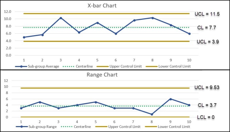
Statistics is the language of uncertainty, where raw numbers transform into actionable insights. At its heart lies a deceptively simple symbol: x̄ (pronounced "x-bar"), the arithmetic mean of a sample. Yet this unassuming notation is the linchpin of modern inference—bridging the gap between observed data and broader truths. Without it, fields from medicine to economics would lack the precision to validate hypotheses or predict trends. The question "what is x bar in statistics" isn’t just academic; it’s the foundation upon which entire industries build confidence in their conclusions.
Consider clinical trials where researchers measure drug efficacy. The raw blood pressure readings of 50 patients are meaningless until aggregated into x̄, the sample mean. This single value becomes the proxy for the population’s response, enabling regulators to approve or reject treatments. Similarly, in quality control, manufacturers rely on x̄ to detect deviations in production lines before defects escalate. The power of x̄ lies in its dual role: as a descriptor of central tendency and as a gateway to statistical inference.
Yet for all its utility, x̄ is often misunderstood. Many conflate it with the population mean (μ), or overlook its sensitivity to outliers. Others dismiss it as mere arithmetic when, in reality, it’s the cornerstone of t-tests, ANOVA, and regression analysis. To wield it effectively—whether in academic research or corporate analytics—requires grasping not just its calculation but its theoretical underpinnings. This guide dissects what is x bar in statistics, from its historical roots to its modern applications, and why mastering it separates novice analysts from those who drive data-driven decisions.
The Complete Overview of What Is X Bar in Statistics
The sample mean, denoted x̄, is the arithmetic average of a subset of data drawn from a larger population. While it shares the same formula as the population mean (μ = ΣX/N), x̄ serves a distinct purpose: estimating μ when examining the whole population is impractical. For instance, if a pollster surveys 1,200 voters instead of all 200 million citizens, x̄ becomes the best available estimate of the population’s true sentiment. This estimation is probabilistic—x̄ will vary slightly with each sample due to sampling error, but its consistency (via the Central Limit Theorem) allows statisticians to quantify uncertainty.
Beyond estimation, x̄ is the bedrock of inferential statistics. It appears in confidence intervals (e.g., "We are 95% confident μ lies between x̄ ± 1.96σ/√n"), hypothesis tests (e.g., comparing x̄ to a known μ), and even non-parametric methods when transformed. Its versatility stems from two properties: (1) it minimizes the sum of squared deviations from all data points (a property known as "least squares"), and (2) it’s unbiased—over infinite samples, the average of all x̄ values will converge to μ. These traits make it indispensable in fields where precision matters, from pharmaceutical trials to financial risk modeling.
Historical Background and Evolution
The concept of averaging data predates modern statistics, but x̄ as a formal tool emerged in the 18th century alongside the rise of probability theory. Carl Friedrich Gauss’s work on the normal distribution in the early 1800s cemented the idea that sample means follow predictable patterns, even when the underlying population is unknown. However, it was Sir Ronald Fisher in the 1920s who elevated x̄ to its current status by developing the framework for statistical inference—using sample means to make inferences about populations. His t-distribution, for instance, provided a way to estimate μ when sample sizes are small, further solidifying x̄’s role.
Table of Contents
- The Complete Overview of What Is X Bar in Statistics
- Historical Background and Evolution
- Core Mechanisms: How It Works
- Key Benefits and Crucial Impact
- Major Advantages
- Comparative Analysis
- Future Trends and Innovations
- Conclusion
- Comprehensive FAQs
- Q: How does x̄ differ from the population mean (μ)?
- Q: Why is the Central Limit Theorem important for x̄?
- Q: Can x̄ be used with non-numeric data?
- Q: How do outliers affect x̄?
- Q: What is the relationship between x̄ and standard error?
- Q: How is x̄ used in hypothesis testing?
- Q: Are there alternatives to x̄ for small sample sizes?
- Q: Can x̄ be negative?
- Q: How does x̄ relate to regression analysis?
- Q: What are common mistakes when calculating x̄?
By the mid-20th century, what is x bar in statistics had become a cornerstone of applied research. The advent of computers in the 1960s democratized its use, allowing industries to compute x̄ for massive datasets efficiently. Today, x̄ is not just a theoretical construct but a practical tool in machine learning (e.g., calculating batch means in deep learning), quality control (e.g., Six Sigma processes), and even social sciences (e.g., measuring average test scores). Its evolution reflects a broader shift: from descriptive statistics to predictive analytics, where x̄ often serves as the first step in building more complex models.
Core Mechanisms: How It Works
The calculation of x̄ is straightforward: sum all observations in a sample and divide by the number of observations (n). For example, if a dataset contains [12, 15, 14, 13], x̄ = (12 + 15 + 14 + 13)/4 = 13.6. However, its statistical power lies in understanding how this single value behaves across repeated samples. The Central Limit Theorem (CLT) states that, regardless of the population distribution, the sampling distribution of x̄ will approximate a normal distribution as n increases—provided the sample size is sufficiently large (typically n ≥ 30). This property allows statisticians to apply normal distribution techniques (e.g., z-tests) even when the original data is skewed.
Yet x̄’s reliability hinges on two critical assumptions: random sampling and independence. If data is collected non-randomly (e.g., surveying only social media users), x̄ may be biased. Similarly, dependent observations (e.g., time-series data) inflate variance, reducing the precision of x̄ as an estimator. Advanced methods like bootstrapping or stratified sampling address these issues, but the core principle remains: x̄ is only as valid as the data it summarizes. This interplay between calculation and context explains why what is x bar in statistics is more than arithmetic—it’s a reflection of study design quality.
Key Benefits and Crucial Impact
The sample mean’s influence extends beyond academia. In healthcare, x̄ determines dosage guidelines; in manufacturing, it triggers corrective actions when production metrics deviate. Even everyday decisions—like choosing a restaurant based on average reviews—rely implicitly on x̄. Its impact stems from three pillars: simplicity, scalability, and statistical rigor. Unlike complex metrics, x̄ is intuitive yet mathematically robust, making it accessible to non-experts while remaining precise enough for rigorous analysis. This duality explains its ubiquity across disciplines.
Critics argue that x̄ can obscure important nuances, such as distribution shape or outliers. However, its advantages often outweigh these limitations. For instance, in A/B testing, x̄ for conversion rates is the primary metric for determining which campaign performs better. The trade-off—ignoring variability for clarity—is justified when the goal is actionable insight. As one statistician noted:
"Statistics is the art of summarizing information while retaining its essence. X̄ is the purest form of this art: it distills complexity into a single number that, when interpreted correctly, speaks volumes."
— George E. P. Box, Statistician and Quality Control Pioneer
Major Advantages
- Unbiased Estimation: Over infinite samples, x̄ will equal the true population mean (μ), ensuring long-term accuracy.
- Foundation for Inference: Enables hypothesis testing (e.g., t-tests) and confidence intervals, which are critical for decision-making.
- Robustness via CLT: Works reliably even with non-normal populations, provided sample sizes are adequate.
- Interpretability: A single value (x̄) is easier to communicate than raw data, aiding stakeholder buy-in.
- Scalability: Computationally efficient for large datasets, making it viable in big data applications.

Comparative Analysis
While x̄ is the most common measure of central tendency, other statistics serve distinct purposes. Understanding their differences clarifies when to use x̄ and when alternatives are better suited.
| Metric | Use Case |
|---|---|
| Sample Mean (x̄) | Estimating population mean (μ); hypothesis testing; confidence intervals. |
| Median | Resistant to outliers; preferred for skewed distributions (e.g., income data). |
| Mode | Identifying most frequent value; useful for categorical data. |
| Trimmed Mean | Reducing outlier impact while retaining central tendency. |
For example, in a dataset with extreme values (e.g., housing prices), the median may better represent "typical" values than x̄. Conversely, x̄ is irreplaceable when the goal is to estimate μ for parametric tests. The choice hinges on data characteristics and analytical objectives.
Future Trends and Innovations
The role of x̄ is evolving alongside data science. Traditional statistical methods are being augmented by machine learning, where x̄ often serves as a baseline feature (e.g., average user engagement scores). In Bayesian statistics, x̄ is incorporated into prior distributions to refine posterior estimates. Meanwhile, high-dimensional data (e.g., genomics) demands extensions of x̄, such as multivariate means or robust alternatives like the M-estimator. These trends reflect a broader shift: x̄ is no longer a standalone metric but a building block in complex models.
Another frontier is real-time analytics, where x̄ is computed dynamically (e.g., streaming sensor data). Here, techniques like exponential smoothing adjust x̄ to account for temporal trends, blending classical statistics with modern computational power. As data grows more heterogeneous, the question "what is x bar in statistics" may expand to include contextualized means—tailored not just to sample size but to the specific problem domain. The future of x̄ lies in its adaptability to these emerging challenges.

Conclusion
What is x bar in statistics is more than a formula—it’s the bridge between raw data and meaningful conclusions. From its origins in 18th-century probability to its current role in AI-driven analytics, x̄ has remained a constant because it solves a fundamental problem: summarizing variability into a single, actionable number. Its limitations (sensitivity to outliers, reliance on random sampling) are outweighed by its versatility, making it the workhorse of statistical inference.
Mastering x̄ isn’t about memorizing calculations; it’s about understanding its implications. Whether you’re validating a clinical trial, optimizing a supply chain, or interpreting survey results, x̄ is the first step in turning data into decisions. As methodologies advance, its principles endure—a testament to the enduring relevance of classical statistics in an era of big data.
Comprehensive FAQs
Q: How does x̄ differ from the population mean (μ)?
A: X̄ is calculated from a sample and estimates μ, while μ is the true average of the entire population. X̄ varies between samples due to sampling error, whereas μ is fixed (though often unknown). For example, if you survey 100 people about their annual income, x̄ might be $50,000, but μ (the average for all citizens) could be $52,000.
Q: Why is the Central Limit Theorem important for x̄?
A: The CLT ensures that, regardless of the population distribution, the sampling distribution of x̄ will be approximately normal if the sample size is large (n ≥ 30). This allows statisticians to use normal distribution techniques (e.g., z-tests) even when the original data is skewed, making x̄ a reliable estimator.
Q: Can x̄ be used with non-numeric data?
A: No. X̄ requires numeric data because it involves arithmetic operations (summation and division). For categorical data (e.g., colors, survey responses), use the mode or proportions instead. However, ordinal data (e.g., Likert scale responses) can sometimes be treated as numeric if intervals are meaningful.
Q: How do outliers affect x̄?
A: X̄ is highly sensitive to outliers because it includes every data point in its calculation. A single extreme value can disproportionately shift x̄, leading to misleading estimates of μ. Robust alternatives like the median or trimmed mean are preferred in such cases.
Q: What is the relationship between x̄ and standard error?
A: The standard error (SE) of x̄ measures its variability across samples and is calculated as SE = σ/√n (where σ is the population standard deviation). A smaller SE indicates that x̄ is a more precise estimator of μ. In practice, SE is often estimated using the sample standard deviation (s) when σ is unknown.
Q: How is x̄ used in hypothesis testing?
A: In tests like the one-sample t-test, x̄ is compared to a hypothesized population mean (μ₀). The test statistic (t = (x̄ – μ₀)/(s/√n)) determines whether to reject μ₀. For example, if x̄ = 45 and μ₀ = 50 with a p-value < 0.05, you’d reject the null hypothesis that the population mean equals 50.
Q: Are there alternatives to x̄ for small sample sizes?
A: Yes. For small samples (n < 30) with unknown population variance, the t-distribution replaces the normal distribution in confidence intervals and hypothesis tests. This adjusts for the greater uncertainty in x̄ when sample sizes are limited. Non-parametric methods (e.g., Wilcoxon signed-rank test) may also be used if data violates normality assumptions.
Q: Can x̄ be negative?
A: Yes, if the data contains negative values. For example, if a dataset of temperature changes includes -2°C, -1°C, and 0°C, x̄ = (-2 + -1 + 0)/3 = -1°C. The sign of x̄ depends solely on the data’s values, not on statistical conventions.
Q: How does x̄ relate to regression analysis?
A: In linear regression, x̄ and the mean of the predictor variable (X̄) are used to calculate predicted values (Ŷ = β₀ + β₁X). The regression line always passes through the point (X̄, Ȳ), ensuring the model’s predictions are centered on the data’s average. This property helps interpret coefficients and assess model fit.
Q: What are common mistakes when calculating x̄?
A: Common errors include:
- Forgetting to divide by n (sample size) instead of N (population size).
- Including non-numeric data (e.g., text labels) in calculations.
- Assuming x̄ represents the entire population without accounting for sampling bias.
- Ignoring units (e.g., reporting x̄ as "5" instead of "5 kg").
Leave a Comment
Comments are moderated before appearing. The data you submit is processed according to the Privacy Policy of Sac.